Getting started with XGI#
![]()
XGI is a Python library to make working with and analyzing complex systems with higher-order interactions easy. We have collected a lot of useful functions, algorithms, and tools for working with hypergraphs and simplicial complexes to make life easier.
We will
Create and load hypergraphs
Visualize hypergraphs and simplicial complexes
Show how to use the stats interface
Give an example of how to compare an empirical dataset to a null model.
We start off by loading the XGI library.
[1]:
import matplotlib.pyplot as plt
import networkx as nx
import numpy as np
import pandas as pd
from IPython.display import display
from matplotlib.pyplot import cm

import xgi
You can easily check the version of XGI that you have installed by using the __version__ property:
[2]:
xgi.__version__
[2]:
'0.9.4'
Creating a hypergraph#
We want to start with a hypergraph, and this can be done in several ways:
Build a hypergraph node-by-node and edge-by-edge (less common, but can be helpful in writing your own generative models)
Load an existing dataset
Sample from a random generative model
Let’s start with the first method.
Building a hypergraph#
[3]:
H_build = xgi.Hypergraph()
H_build.add_edge([1, 2], idx="a")
H_build.add_node(0)
H_build.add_edges_from([[3, 4], [0, 2, 3]])
H_build.add_nodes_from([9, 10])
XGI automatically assigns unique edge IDs (if a user doesn’t specify the ID)
[4]:
H_build.edges
[4]:
EdgeView(('a', 0, 1))
Why NodeViews and EdgeViews? These allow users to access many different properties and data structures from nodes and edges in a much simpler way. We will cover this more in depth later. For now, we can get the edges of which each node is a part and the nodes in each edge as follows:
[5]:
H_build.edges
[5]:
EdgeView(('a', 0, 1))
[6]:
print(H_build.nodes.memberships())
print(H_build.edges.members())
print(H_build.nodes.memberships(2))
print(H_build.edges.members("a"))
{1: {'a'}, 2: {1, 'a'}, 0: {1}, 3: {0, 1}, 4: {0}, 9: set(), 10: set()}
[{1, 2}, {3, 4}, {0, 2, 3}]
{1, 'a'}
{1, 2}
Loading datasets#
Moving on to method 2, one can load datasets in several different ways. First, we provide a companion data repository, xgi-data, where users can easily load several datasets in standard format:
[7]:
H_enron = xgi.load_xgi_data("email-enron")
This dataset, for example, has a corresponding datasheet explaining its characteristics. The nodes (individuals) in this dataset contain associated email addresses and the edges (emails) contain associated timestamps. These attributes can be accessed by simply typing H.nodes[id] or H.edges[id] respectively.
[8]:
print(f"The hypergraph has {H_enron.num_nodes} nodes and {H_enron.num_edges} edges")

# We can also print a summary of the hypergraph
print(H_enron)
The hypergraph has 148 nodes and 10885 edges
Hypergraph named email-Enron with 148 nodes and 10885 hyperedges
[9]:
print("The first 10 node IDs are:")
print(list(H_enron.nodes)[:10])
print("\nThe first 10 edge IDs are:")
print(list(H_enron.edges)[:10])
print("\nThe attributes of node '4' are")
print(H_enron.nodes["4"])
print("\nThe attributes of edge '6' are")
print(H_enron.edges["6"])
The first 10 node IDs are:
['4', '1', '117', '129', '51', '41', '65', '107', '122', '29']

The first 10 edge IDs are:
['0', '1', '2', '3', '4', '5', '6', '7', '8', '9']

The attributes of node '4' are
{'name': 'robert.badeer@enron.com'}

The attributes of edge '6' are
{'timestamp': '2000-02-22T08:07:00'}
We can clean up this dataset to remove isolates, multi-edges, singletons, and to replace all IDs with integer IDs.
[10]:
H_enron_cleaned = H_enron.cleanup(
    multiedges=False, singletons=False, isolates=False, relabel=True, in_place=False
)

print(H_enron_cleaned)

print("The first 10 node IDs are:")
print(list(H_enron_cleaned.nodes)[:10])
Hypergraph named email-Enron with 143 nodes and 1459 hyperedges
The first 10 node IDs are:
[0, 1, 2, 3, 4, 5, 6, 7, 8, 9]
Random null models#
Lastly, we can create synthetic hypergraphs using random generative models. For example, we can extract the degree and edge size sequence from this dataset and wire them together at random (according to the Chung-Lu model) to create a random null model:
[11]:
D = H_enron_cleaned.dual()
k = H_enron_cleaned.nodes.degree.asdict()
s = H_enron_cleaned.edges.size.asdict()

H_random = xgi.chung_lu_hypergraph(k, s)
We check whether this new hypergraph is connected and if not, the sizes of the connected components:
[12]:
connected = xgi.is_connected(H_random)
if not connected:
    size, num = np.unique(
        [len(cc) for cc in xgi.connected_components(H_random)], return_counts=True
    )
    print(size)
    print(num)
    print("The connected components:")
    display(pd.DataFrame([size, num], columns=["Component size", "Number"]))
[  1 141]
[2 1]
The connected components:
| Component size | Number | |
|---|---|---|
| 0 | 1 | 141 |
| 1 | 2 | 1 |
Converting between different representations#
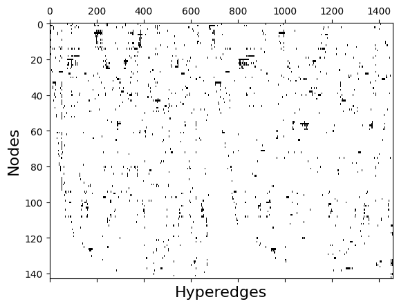
Incidence matrix#
Any hypergraph can be expressed as an \(N \times M\) incidence matrix, \(I\), where \(N\) is the number of nodes and \(M\) is the number of edges. Rows indicate the node ID and the columns indicate the edge ID. \(I_{i,j}=1\) if node \(i\) is a member of edge \(j\) and zero otherwise.
[13]:
I = xgi.incidence_matrix(H_enron_cleaned, sparse=False)
plt.spy(I, aspect="auto")
plt.xlabel("Hyperedges", fontsize=16)
plt.ylabel("Nodes", fontsize=16)
plt.show()
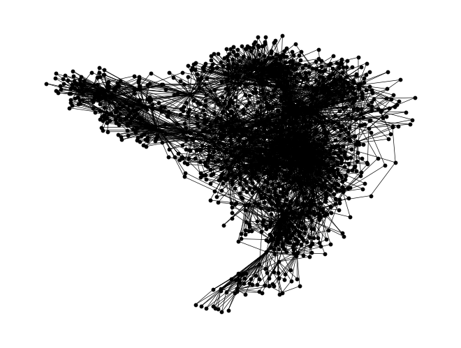
Bipartite network#
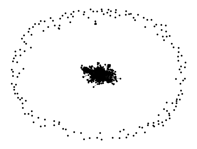
Any hypergraph can be mapped to an equivalent bipartite network, \(G\), where nodes become nodes of the first type and edges become nodes of the second type. A bipartite link \((i, j)\) of \(G\) indicates that node \(i\) is a member of edge \(j\).
[14]:
G = xgi.to_bipartite_graph(H_enron_cleaned)
nx.draw(G, node_color="black", node_size=10, width=0.5)
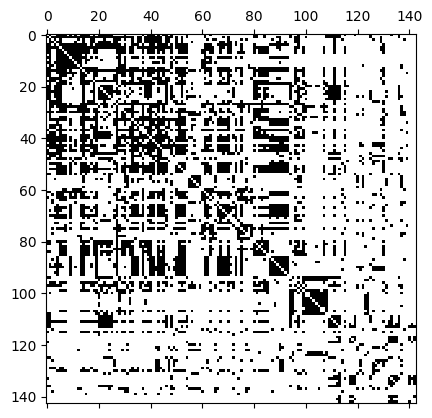
Adjacency matrix#
We can represent a hypergraph with an \(N\times N\) adjacency matrix, \(A\), where \(N\) is the number of nodes. The adjacency matrix is a lossy format; different hypergraphs can create the same adjacency matrix. \(A_{i,j} = 1\) if there is at least one hyperedge containing both nodes \(i\) and \(j\).
[15]:
A = xgi.adjacency_matrix(H_enron_cleaned, sparse=False)
plt.spy(A)
[15]:
<matplotlib.image.AxesImage at 0x72b7b6f9ef10>
Line graph#
The \(s\)-line graph is a network where nodes are hyperedges and a link is formed between two edges if they share at least \(s\) nodes in common.
[16]:
G = xgi.to_line_graph(H_enron_cleaned, s=2)
nx.draw(G, node_color="black", node_size=10, width=0.5)
The dual#
The dual is a hypergraph whose vertices and edges are interchanged. This can be pictured by swapping the nodes of the first and second types in the bipartite representation.
[17]:
D = H_enron_cleaned.dual()
print(D)
Hypergraph named email-Enron with 1459 nodes and 143 hyperedges
We can do much more such as computing different properties, reading/writing, converting to/from different data structures, hypergraph null models and much more!
See the Read The Docs for more information: https://xgi.readthedocs.io
Visualization#
The first step for drawing a hypergraph is to choose a layout for the nodes. At the moment the available layouts are:
random_layout: positions nodes uniformly at random in the unit square.pairwise_spring_layout: positions the nodes using the Fruchterman-Reingold force-directed algorithm on the projected graph.barycenter_spring_layoutandweighted_barycenter_spring_layout: slight modification ofpairwise_spring_layout
Each layout returns a dictionary that maps nodes ID into (x, y) coordinates.
[18]:
seed = 0
H_viz = xgi.random_hypergraph(20, [0.08, 0.01, 0.001], seed=seed)
pos1 = xgi.random_layout(H_viz)
pos2 = xgi.pairwise_spring_layout(H_viz)
pos3 = xgi.barycenter_spring_layout(H_viz)
pos4 = xgi.weighted_barycenter_spring_layout(H_viz)
/home/lucasm/WORK/SCIENCE/xgi/xgi/generators/random.py:154: UserWarning: This method is much slower than fast_random_hypergraph
  warn("This method is much slower than fast_random_hypergraph")
[19]:
xgi.draw(H_viz, pos1)
[19]:
(<Axes: >,
 (<matplotlib.collections.PathCollection at 0x72b7b7191d10>,
  <matplotlib.collections.LineCollection at 0x72b7b6e2e3d0>,
  <matplotlib.collections.PatchCollection at 0x72b7b717f850>))
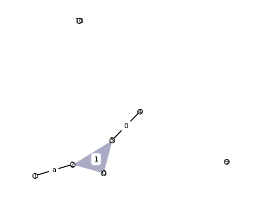
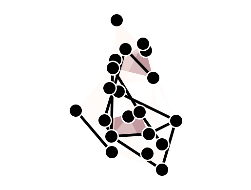
We can easily add labels to the nodes to more easily compare the visualization to the hypergraph:
[20]:
xgi.draw(H_build, node_labels=True, hyperedge_labels=True)
[20]:
(<Axes: >,
 (<matplotlib.collections.PathCollection at 0x72b7b717bad0>,
  <matplotlib.collections.LineCollection at 0x72b7bcbf1110>,
  <matplotlib.collections.PatchCollection at 0x72b7b7179c90>))
Colors of the hyperedges are designed to match the hyperedge size, but the colormap can be tweaked:
[21]:
# Sequential colormap
cmap = cm.Paired

xgi.draw(H_viz, pos4, edge_fc_cmap=cmap)
[21]:
(<Axes: >,
 (<matplotlib.collections.PathCollection at 0x72b7b736bbd0>,
  <matplotlib.collections.LineCollection at 0x72b7b6e2fd50>,
  <matplotlib.collections.PatchCollection at 0x72b7b6f7ca10>))
Other parameters can be changed as well:
[22]:
cmap = cm.Reds
dyad_lc = "gray"
dyad_lw = 4
node_fc = "black"
node_ec = "white"
node_lw = 2
node_size = 20

xgi.draw(
    H_viz,
    pos4,
    edge_fc_cmap=cmap,
    dyad_lc=dyad_lc,
    dyad_lw=dyad_lw,
    node_fc=node_fc,
    node_ec=node_ec,
    node_lw=node_lw,
    node_size=node_size,
)
[22]:
(<Axes: >,
 (<matplotlib.collections.PathCollection at 0x72b7b6fcbc50>,
  <matplotlib.collections.LineCollection at 0x72b7b6fc5090>,
  <matplotlib.collections.PatchCollection at 0x72b7b6d03cd0>))
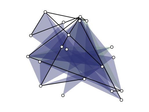
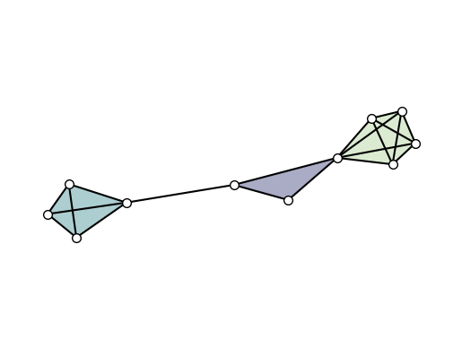
Simplicial complexes can be visualized using the same functions for node layout and drawing.
Technical note#
By definition, a simplicial complex object contains all sub-simplices. This would make the visualization heavy since all sub-simplices contained in a maximal simplex would overlap. The automatic solution for this, implemented by default in all the layouts, is to convert the simplicial complex into a hypergraph composed by solely by its maximal simplices.
Visual note#
To visually distinguish simplicial complexes from hypergraphs, the draw function will also show all links contained in each maximal simplices (while omitting simplices of intermediate orders).
[23]:
SC = xgi.SimplicialComplex()
SC.add_simplices_from([[3, 4, 5], [3, 6], [6, 7, 8, 9], [1, 4, 10, 11, 12], [1, 4]])

pos = xgi.pairwise_spring_layout(SC)
xgi.draw(SC, pos)
[23]:
(<Axes: >,
 (<matplotlib.collections.PathCollection at 0x72b7bc111c90>,
  <matplotlib.collections.LineCollection at 0x72b7b6f9d690>,
  <matplotlib.collections.PatchCollection at 0x72b7b6d9ab10>))
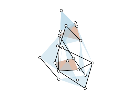
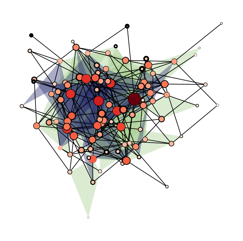
We can even color/draw the nodes and edges based on statistics!
[24]:
n = 100
is_connected = False
while not is_connected:
    H = xgi.random_hypergraph(n, [0.03, 0.0002, 0.00001])
    is_connected = xgi.is_connected(H)
pos = xgi.barycenter_spring_layout(H)
/home/lucasm/WORK/SCIENCE/xgi/xgi/generators/random.py:154: UserWarning: This method is much slower than fast_random_hypergraph
  warn("This method is much slower than fast_random_hypergraph")
[25]:
plt.figure(figsize=(10, 10))
ax = plt.subplot(111)
xgi.draw(
    H,
    pos,
    node_size=H.nodes.degree,
    node_lw=H.nodes.average_neighbor_degree,
    node_fc=H.nodes.degree,
    ax=ax,
)
[25]:
(<Axes: >,
 (<matplotlib.collections.PathCollection at 0x72b7bcbf8150>,
  <matplotlib.collections.LineCollection at 0x72b81c1566d0>,
  <matplotlib.collections.PatchCollection at 0x72b7affdd010>))
The stats package#
The stats package is one of the features that sets xgi apart from other libraries. It provides a common interface to all statistics that can be computed from a network, its nodes, or edges.
Consider the degree of the nodes of a hypergraph H. After computing the values of the degrees, one may wish to store them in a dict, a list, an array, a dataframe, etc. Through the stats package, xgi provides a simple interface that seamlessly allows for this type conversion. This is done via the NodeStat class.
[26]:
import numpy as np
import pandas as pd

import xgi

H_stats = xgi.Hypergraph([[1, 2, 3], [2, 3, 4, 5], [3, 4, 5]])
H_stats.degree()
[26]:
{1: 1, 2: 2, 3: 3, 4: 2, 5: 2}
[27]:
H_stats.nodes.degree
[27]:
NodeStat('degree')
This NodeStat object allows us to choose the datatype, specify keywords, and get basic statistics from these properties
[28]:
print("As a dictionary:")
print(H_stats.nodes.degree.asdict())
print("\nAs a list:")
print(H_stats.nodes.degree.aslist())
print("\nAs a numpy array:")
print(H_stats.nodes.degree.asnumpy())
print("\nAs a pandas dataframe:")
print(H_stats.nodes.degree.aspandas())
As a dictionary:
{1: 1, 2: 2, 3: 3, 4: 2, 5: 2}

As a list:
[1, 2, 3, 2, 2]

As a numpy array:
[1 2 3 2 2]

As a pandas dataframe:
1    1
2    2
3    3
4    2
5    2
Name: degree, dtype: int64
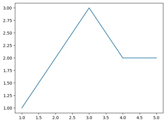
[29]:
H_stats.nodes.degree.aspandas().plot()
[29]:
<Axes: >
[30]:
print(H_stats.nodes.degree(order=2).asdict())
{1: 1, 2: 1, 3: 2, 4: 1, 5: 1}
[31]:
st = H_stats.nodes.degree
np.round([st.max(), st.min(), st.mean(), st.median(), st.var(), st.std()], 3)
[31]:
array([3. , 1. , 2. , 2. , 0.4 , 0.632])
Likewise, for edges,
[32]:
st = H_stats.edges.size
st
[32]:
EdgeStat('size')
[33]:
np.round([st.max(), st.min(), st.mean(), st.median(), st.var(), st.std()], 3)
[33]:
array([4. , 3. , 3.333, 3. , 0.222, 0.471])
The interface for attributes is very similar. If we add nodal attributes, for example
[34]:
H_stats.add_nodes_from(
    [
        (1, {"color": "red", "name": "horse"}),
        (2, {"color": "blue", "name": "pony"}),
        (3, {"color": "yellow", "name": "zebra"}),
        (4, {"color": "red", "name": "orangutan", "age": 20}),
        (5, {"color": "blue", "name": "fish", "age": 2}),
    ]
)
print(H_stats.nodes.attrs("color").asdict())
{1: 'red', 2: 'blue', 3: 'yellow', 4: 'red', 5: 'blue'}
[35]:
print(H_stats.nodes.attrs[1])
{'color': 'red', 'name': 'horse'}
One can also filter nodes and edges by their attributes as well as any associated statistic. For example,
[36]:
print(H_stats.nodes.filterby("degree", 2))
print(H_stats.nodes.filterby_attr("color", "blue"))
[2, 4, 5]
[2, 5]
[37]:
H_stats.edges.filterby("size", 3).members()
[37]:
[{1, 2, 3}, {3, 4, 5}]
[38]:
H_stats.nodes.multi(["degree", "clustering_coefficient"]).aspandas().groupby(
    "degree"
).agg("mean")
[38]:
| clustering_coefficient | |
|---|---|
| degree | |
| 1 | 1.000000 |
| 2 | 0.888889 |
| 3 | 0.666667 |
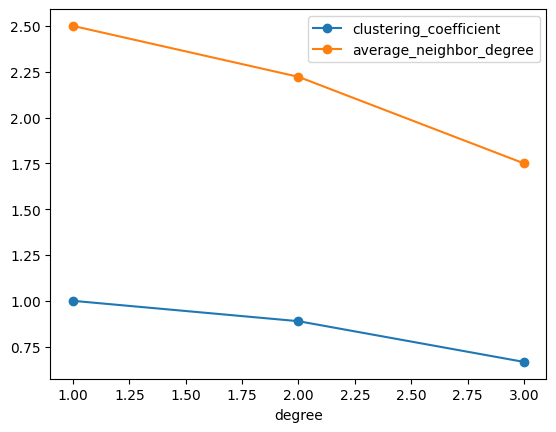
[39]:
(
    H_stats.nodes.multi(["degree", "clustering_coefficient", "average_neighbor_degree"])
    .aspandas()
    .groupby("degree")
    .agg("mean")
    .plot(marker="o")
)
[39]:
<Axes: xlabel='degree'>
For even more functionality, see the Read The Docs: https://xgi.readthedocs.io
Let’s compare the assortativity of an empirical dataset (Let’s choose the email-enron dataset) to a random null model. We start by loading the Enron dataset and constructing a Chung-Lu hypergraph using the dataset’s degree sequence and edge size sequence:
[40]:
H = H_enron
k = H.nodes.degree.asdict()
s = H.edges.size.asdict()

H_null = xgi.chung_lu_hypergraph(k, s)
Now we use the definitions of assortativity in “Configuration models of random hypergraphs” by Phil Chodrow to compare the assortativity of the random null model to the original dataset.
[41]:
labels = ["uniform", "top-2", "top-bottom"]

assort_orig = []
assort_null = []
for l in labels:
    assort_orig.append(xgi.degree_assortativity(H, kind=l))
    assort_null.append(xgi.degree_assortativity(H_null, kind=l))

x = np.arange(len(labels))
width = 0.35

fig, ax = plt.subplots()
rects1 = ax.bar(x - width / 2, assort_orig, width, label="Original")
rects2 = ax.bar(x + width / 2, assort_null, width, label="Null model")
ax.set_xticks(x)
ax.set_xticklabels(labels, fontsize=16)
ax.set_ylabel("Assortativity", fontsize=16)
ax.legend()
plt.tight_layout()
plt.show()
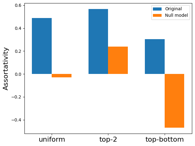
From this plot we can see that the original dataset is more assortative than the random null model.
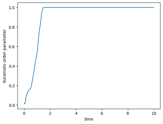
Dynamics#
We can also simulate the order parameter of the Kuramoto model for hypergraphs.
[42]:
n = 100
H = xgi.random_hypergraph(n, [0.05, 0.001], seed=None)
omega = 2 * np.random.normal(1, 0.05, n)
theta = np.linspace(0, 2 * np.pi, n)
timesteps = 1000
dt = 0.01

theta, t = xgi.simulate_kuramoto(
    H, k2=2, k3=3, omega=omega, theta=theta, timesteps=timesteps, dt=dt
)
R = xgi.compute_kuramoto_order_parameter(theta)
/home/lucasm/WORK/SCIENCE/xgi/xgi/generators/random.py:154: UserWarning: This method is much slower than fast_random_hypergraph
  warn("This method is much slower than fast_random_hypergraph")
[43]:
plt.figure()
plt.plot(t, R)
plt.xlabel("time")
plt.ylabel("Kuramoto order parameter")
plt.show()